Causal Normalizing Flow

In this blog post we discuss the idea of using normalizing flow for cause-effect discovery and multivariate causal discovery with results of three different normalizing flows on two datasets.

Introduction to Causal discovery

Causal inference has an important role in different areas including machine learning, providing new modelings that can answer new prediction tasks. In order to do causal inference, we need to discover causal relationships between variables.

There are two approaches for causal discovery including constraint and score-based. Constraint-based methods use conditional independence tests in the joint distribution and so these methods output CPDAGs or a graph which belongs to a Markov equivalence class. The problem with these methods is that independence tests need large sample sizes to be reliable. The most well known methods are Spirtes-Glymour-Scheines (SGS), Peter-Clark (PC) and Fast Causal Inference (FCI) [1]. In contrast score-based approaches test the validity of a candidate graph G according to some scoring function $S$

$argmax_{G}$ $S(D, G)$

where $D$ represents the observational samples for variables. The most well known function S is bayesian information criteria (BIC).

In this article we are going to use normalizing flow as a likelihood-based method for causal discovery. First, we discuss the two-variable case where we want to find which variable is cause and which one is effect. After that, we examine methods and research directions in which we can discover causal relationships between variables using normalizing flow and compare it with other neural causal discovery methods.

Cause Effect Discovery Using normalizing flow

The task of cause-effect discovery is the decision between two causal model X->Y or Y->X One score function for choosing from these two models is likelihood ratio [2], [3]. Also normalizing flow is a likelihood based model which can be used as a score function for causal discovery. Following the Causal Autoregressive flow [4] we implement a normalizing flow in pytorch to see how NF behaves between two mentioned causal models. After that we will try to investigate if we can extend NF to multivariate-case comparing it to other neural causal models including Gradient-based Neural Dag Learning [5] and Learning sparse nonparametric dags [6].

Normalizing flow

Normalizing flow is a density estimation method which learns complex probability distributions by transforming a simple distribution, for example a gaussian distribution, to a complex one. NF does this by applying a series of transformations f and using change of variables theorem we can compute the exact likelihood of complex distribution, Fig 1. Examples of such transformations are RealNVP [7], Nice [8], and GLOW [9]. We will use RealNVP in this tutorial. For a complete introduction to normalizing flow read the great blog post by Weng, Lilian about Flow-based Deep Generative Models.

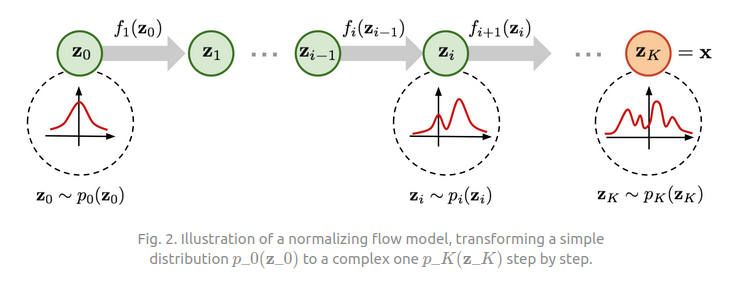
[10] Weng, Lilian, 2018, Flow-based Deep Generative Models. Lilianweng.github.io.

Causal normalizing flow

In this section we want to compare the learned distribution of two datasets. Two data sets are a non-causal dataset (moon dataset) and a causal dataset generated from a structure equation model.

Below there are the equations and the plot of the generated data for two datasets:

Moon dataset:

outer_circ_x = np.cos(np.linspace(0, np.pi, 100))
outer_circ_y = np.sin(np.linspace(0, np.pi, 100))
inner_circ_x = 1 - np.cos(np.linspace(0, np.pi, 100))
inner_circ_y = 1 - np.sin(np.linspace(0, np.pi, 100)) - 0.5

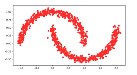
Fig 2, Moon dataset.

Causal dataset:

$X$ $->$ $Y$
$x = laplace(0, 1/\sqrt{2})$
$y = x + 0.5 * x^3 + laplace(0, 1/\sqrt{2})$

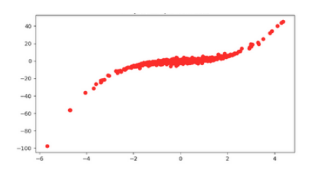
Fig 3, Causal dataset, generated by a structure equation model.

Normalizing Flow models

In real nvp there are multiple transformations in which half of the variables go through the model without changing and the others go through an affine coupling transformation. You can see each transformation below.

To increase the expressiveness of transformation the order of variables changes after each stack of normalizing flow, Fig 4.

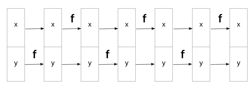
Fig 4, Stack of flows for non-causal dataset (moon dataset): $X-Y$. Order reversed in each stack.

But suppose that we want to learn the distribution of a causal data set $X->Y$. So we might not need to change the order of variables and apply function $F$ on variable $Y$, Fig 5.

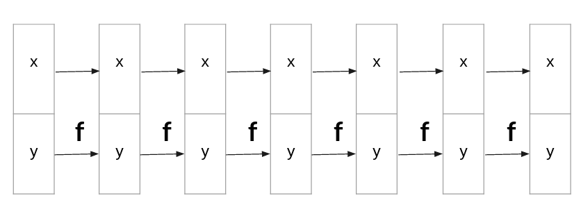
Fig 5, Stack of flows for causal dataset: $X->Y$

And if we want to learn the distribution of data in reverse order $Y->X$ we must apply $F$ to $X$, Fig 6.

Fig 6, Stack of flows for causal dataset: $Y->X$

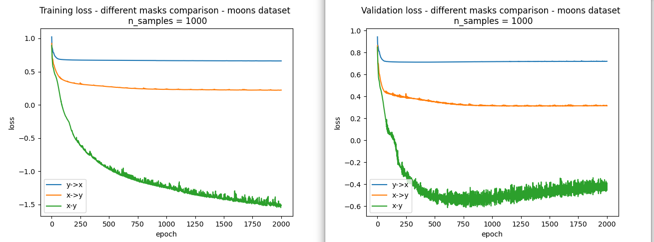
So based on the above two datasets and the three Normalizing flow models, we will train 3 flows on each datasets and compare the results.

Moon dataset:

In Fig 7, training and validation loss of 3 normalizing flow plotted. As you can see the best loss is related to normalizing flow $X-Y$ which reverses order of variables in each stack of flow, thus it learned the distribution of non-causal dataset more accurate.

Causal datasets:

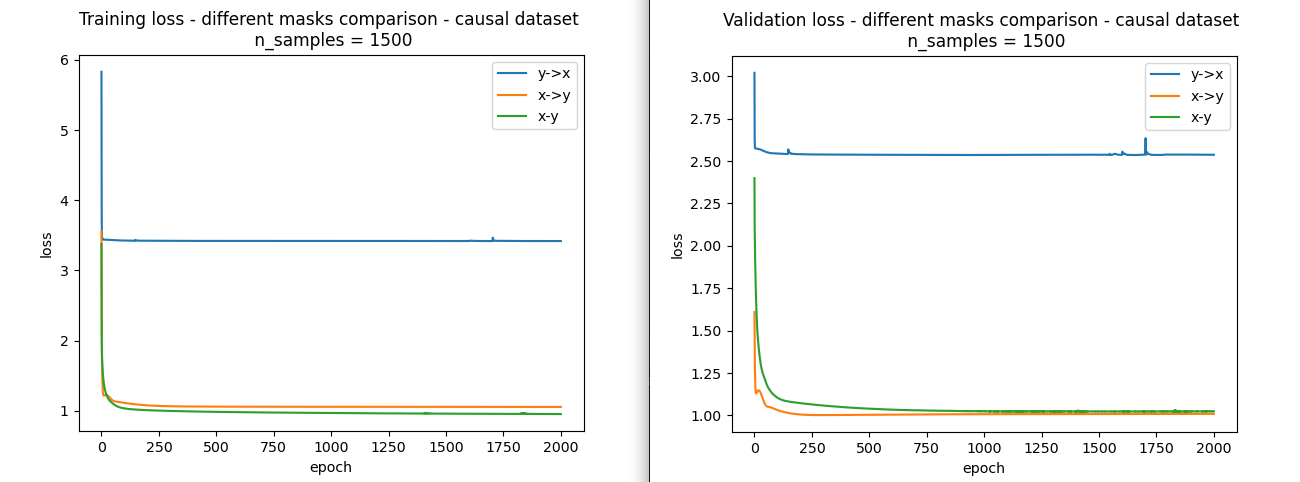
Now, let’s move to the causal dataset and compare the three kinds of norm. As you know, the correct causal direction of this dataset is $X->Y$. So we expect that loss of $X->Y$ reaches the loss of $X-Y$ and is dominantly better than loss of $Y->X$.

As you can see, our hypothesis is correct and if our data generation process follows a causal model it’s not necessary to reverse the order of variables in each stack of flows. Also, We can use likelihood loss as a metric that can recognize the correct order of cause-effect between two variables.

Full implementation is available here.

Multivariate Causal discovery

First, we discuss two approaches for causal discovery that use neural networks like normalizing flow and investigate their problems. After that we discuss if we can use normalizing flow two solve those problems.

Gradient-based Neural Dag Learning [5]

Gran Dag presented a neural network in which defined a constraint that cuts some connectivity paths between weights of the neural network. This constraint forces causal relationship between variables and non-causal relationship between variables has zero weights in the corresponding neural network.
It first defined $C$ as the connectivity path between inputs and outputs variables.

And define the dag constraint on $C$ which is proposed in NO-TEARS [11] and learn a dag by optimizing likelihood of data and satisfying this constraint. (This constraint converted the combinatorial nature of the causal discovery algorithm to a continuous optimization method.)

Learning sparse nonparametric dags [6]

This method defines a neural network for modeling each variable Each neural network $i$ inputs all variables except the $i-th$ variable and outputs the $i-th$ variable. After that to model causal relationship between variables it used the fact that if the $j-th$ column of weights of the first layer of the neural network become zero then the output $i$ is independent of variable $j$. Therefore by satisfying the same constraint like notears it models the causal relationship between all variables.

Gradient-based Neural Dag Learning vs Learning sparse nonparametric dags.

Gran Dag models the causal relationship between variables with just one neural network by satisfying the causal connectivity constraint between weights of the neural network which is definitely hard to find such that constraint. In contrast, Sparse nonparametric dags uses n (number of variables) neural networks but cut dependency between variables by just zeroing out weights of the first layer and satisfying the dag constraint by just weights of first layers of all n neural networks. It seems that this constraint is easier to optimize than Gran-dag which uses weights of all layers of the neural network. But to reach this easier constraint it has to use n neural networks instead of one.

Multivariate Causal discovery with normalizing flow?

I have been researching on this question trying to figure out how can we model causal relationship between multiple variables using normalizing flow which does not have the problem of learning n neural networks instead of one in Sparse nonparametric dags, and hard to optimize dag constraint in Gran Dag.

References

[1] Peter Spirtes, Clark N Glymour, Richard Scheines, and David Heckerman. Causation, prediction, and search. MIT press, 2000.

[2] Zhang, K. and Hyvärinen, A., 2016. Nonlinear functional causal models for distinguishing cause from effect. Statistics and Causality; John Wiley & Sons, Inc.: New York, NY, USA, pp.185-201.

[3] Monti, R.P., Zhang, K. and Hyvärinen, A., 2020, August. Causal discovery with general non-linear relationships using non-linear ica. In Uncertainty in artificial intelligence (pp. 186-195). PMLR.

[4] Khemakhem, I., Monti, R., Leech, R. and Hyvarinen, A., 2021, March. Causal autoregressive flows. In International conference on artificial intelligence and statistics (pp. 3520-3528). PMLR.

[5] Lachapelle, S., Brouillard, P., Deleu, T. and Lacoste-Julien, S., 2019. Gradient-based neural dag learning. arXiv preprint arXiv:1906.02226.

[6] Zheng, X., Dan, C., Aragam, B., Ravikumar, P. and Xing, E., 2020, June. Learning sparse nonparametric dags. In International Conference on Artificial Intelligence and Statistics (pp. 3414-3425). PMLR.

[7] Dinh, L., Sohl-Dickstein, J. and Bengio, S., 2016. Density estimation using real nvp. arXiv preprint arXiv:1605.08803.

[8] Dinh, L., Krueger, D. and Bengio, Y., 2014. Nice: Non-linear independent components estimation. arXiv preprint arXiv:1410.8516.

[9] Kingma, D.P. and Dhariwal, P., 2018. Glow: Generative flow with invertible 1x1 convolutions. Advances in neural information processing systems, 31.

[10] Weng, Lilian, 2018, Flow-based Deep Generative Models. In lilianweng.github.io, Link

[11] Zheng, X., Aragam, B., Ravikumar, P.K. and Xing, E.P., 2018. Dags with no tears: Continuous optimization for structure learning. Advances in Neural Information Processing Systems, 31.